Transformer

In this blog post, we will be going over the Transformer architecture. Introduced by Google in 2017 to solve language translation, Transformers revolutionized natural language processing by replacing recurrent models with an attention-based approach. Since then, Transformer variants have gone on to dominate not only NLP, but also fields like computer vision, speech recognition, and many others.

In this blog post, we will focus on the language translation where we will dive deeper into Vanilla Transformer. In this setup, we will consider English as the source language, while Nepali as the target language that our Transformer aims to predict. The goal of the model is to learn the relationship between source and target sentences so that, given an English sentence, it can generate the corresponding Nepali translation.

In last blog post, we went through different encoding approaches, including Byte Pair Encoding (BPE). However, in this post, I want to keep things simple and use word-level encoding, where each individual word is treated as a token. This makes it easier to understand how Transformers work without getting distracted by more advanced tokenization techniques.

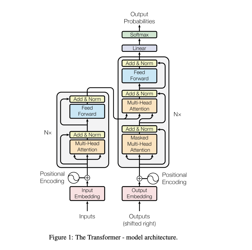
A Transformer consists of two main components: the Encoder and the Decoder. In this post, we will break down each component step by step and understand how information flows through the network. We will also look closely at how the different matrices are transformed and propagated during the forward pass, since matrix operations are at the core of how Transformers work.

Gist of dataset

Since we are working on a language translation, we have corresponding English and Nepali text pairs in our dataset. Each English sentence is the source text, while the corresponding Nepali sentence is the target text

An Example of src text:

mouth is not empty.

Corresponding src text encoding:

[ 2, 0, 9, 19, 0, 4, 3, 1]

An Example of tgt text

मुख खाली थिएन ।

Corresponding tgt text encoding:
[ 2, 0, 668,  92, 4, 1,  1, 1]

Here both source and target have vocab size of 1024 and sequence length of 8

Keeping the numbers small so that it is easy to visualize.

Data Representation

We saw an example of a source and target text with a shape of (1, 8), where 8 represents the sequence length. However, sending only a single example to the model at a time is inefficient. Instead, we group multiple examples together into a batch and pass them through the model simultaneously.

For instance, let’s assume we use a batch size of 2. In that case, our data will have a shape of (2, 8).

Encoder

The encoder processes the source text and generates contextual representations. These encoder outputs, together with the target sequence, are then provided to the decoder to generate the final output token by token.

Input Embeddings

The Transformer model cannot operate directly on int token IDs such as an input tensor of shape (2, 8). These integers are simply indices representing tokens in the vocabulary and contain no semantic meaning by themselves.

To make them useful for the model, each token ID is passed through an embedding layer, which converts it into a dense vector representation.

The Input Embedding layer takes each token and projects it into a higher-dimensional vector space so that the model can learn semantic and contextual relationships. The larger the embedding dimension, the more information the model can potentially capture about each token.

Let’s assume our embedding dimension is 12.

So the transformation becomes:

(2, 8) => [Input Embeddings] => (2, 8, 12)

This means that every token in every sequence is now represented by a vector of size 12 instead of just a single integer token ID.

class InputEmbeddings(nn.Module):

    def __init__(self, emb_dim, vocab_dim):
        super().__init__()
        self.emb_dim = emb_dim
        self.vocab_dim = vocab_dim
        self.embeddings = nn.Parameter(torch.randn(vocab_dim, emb_dim))

    def forward(self, x):
        return self.embeddings[x] * (self.emb_dim) ** (-1/2)

PyTorch already provides nn.Embedding for creating embeddings, but in this post, we will implement the embedding layer manually using nn.Parameter. This allows us to explicitly see how the matrix multiplication works under the hood, making the flow of data through the Transformer much easier to understand. We will follow the same approach for the other layers as well so that every matrix operation becomes transparent.

Positional Embeddings

Since the Transformer processes all tokens in parallel, it has no inherent understanding of the order of words in a sentence. To give the model information about token positions, we add positional embeddings to the input embeddings.

In the original Transformer paper, the authors used sinusoidal positional embeddings, where the positional values are generated using sine and cosine functions. However, instead of using fixed sinusoidal values, we can make the positional embeddings learnable parameters. During training, the model learns these position representations on its own, and in practice, they often converge to patterns similar to sinusoidal embeddings.

From our Input Embeddings we have data shape of (2, 8, 12) then our positional embeddings will also have a shape of (8, 12)

Since the same positional information is shared across all examples in the batch, the positional embeddings are broadcast across the batch dimension and added to the input embeddings:

(2, 8, 12) + (8, 12) => (2, 8, 12)

Now the channel contains both semantic information from token embeddings positional information from positional embeddings

class PositionalEmbeddings(nn.Module):

    def __init__(self, emb_dim, block_size):
        super().__init__()
        self.block_size = block_size
        self.emb_dim = emb_dim
        self.pe = nn.Parameter(torch.randn(block_size, emb_dim))

    def forward(self, x):

        pe = self.pe[0:x.shape[1], :]
        return x+pe

Crux of Transformer: Attention

Attention mechanisms did existed even before Transformers, but they were mostly used alongside RNNs and LSTMs. While attention improved the ability of RNN-based models to capture long-range dependencies, the sequential nature of RNNs still caused problems such as vanishing gradients and exploding gradients, making training difficult for long sequences.

The Transformer paper introduced a major shift by completely removing recurrence and relying entirely on attention mechanisms. This made training significantly more parallelizable and allowed the model to capture long-range relationships much more effectively.

Attention allows each token in a sequence to “talk” to every other token and gather relevant information from them. Instead of processing words one by one like RNNs, attention enables the model to look at the entire sequence at once and determine which tokens are most important for understanding the current token.

Attention works using three learned representations called Queries (Q), Keys (K), and Values (V).

For every token in the sequence, the model generates three vectors:

• a Query vector ; What information am I looking for?
• a Key vector ; What information do I contain?
• a Value vector ; What information should I contribute if I am relevant?

The attention mechanism works by taking the dot product between the Query and Key. This dot product produces attention scores that represent how relevant each token is to the current token.

These scores are then used to compute a weighted aggregation of the Value vector.

This process allows each token to gather contextual information from every other token in the sequence.

class Attention(nn.Module):

    def __init__(self, emb_dim, n_head, head_dim):
        super().__init__()
        self.emb_dim = emb_dim
        self.n_head = n_head
        self.head_dim = head_dim
        self.q = nn.Parameter(torch.randn(emb_dim, emb_dim))
        self.k = nn.Parameter(torch.randn(emb_dim, emb_dim))
        self.v = nn.Parameter(torch.randn(emb_dim, emb_dim))
        self.projection = nn.Parameter(torch.randn(emb_dim, emb_dim))

    @staticmethod
    def attention(q, k, v, mask):
        # q=>(B, H, T, HD)
        # k=>(B, H, T, HD)
        # v=>(B, H, T, HD)

        head_dim = q.shape[-1]
        wei = q @ k.transpose(-2, -1) * (head_dim) **(-1/2)
        # wei=> (B, H, T, HD) @ (B, H, HD, T) => (B, H, T, T)

        if mask is not None:
            wei.masked_fill_(mask==0,float("-inf"))
        wei = wei.softmax(dim=-1)

        # (B, H, T, T)  @ (B, H, T, HD) => (B, H, T, HD)
        return wei@v, wei


    def forward(self, q,k,v, mask):
        B,T,C = q.shape
        q = q @ self.q
        k = k @ self.k
        v = v @ self.v
        q = q.view(q.shape[0], q.shape[1], self.n_head,  self.head_dim).transpose(1,2)
        k = k.view(k.shape[0], k.shape[1], self.n_head,  self.head_dim).transpose(1,2)
        v = v.view(v.shape[0], v.shape[1], self.n_head,  self.head_dim).transpose(1,2)
        out, attn = Attention.attention(q, k, v, mask)
        # out shape=> (B, H, T, HD) => (B, T, H, HD)
        out = out.transpose(1,2).contiguous().view(B, -1, self.emb_dim)
        # (C,C) @ (B, T, C)
        return out @ self.projection

It might be better if we walk through the code step by step to fully understand how attention works.

q = q @ self.q
k = k @ self.k
v = v @ self.v

Here, the inputs are multiplied with learned weight matrices to produce the Query, Key, and Value representations.

(2, 8, 12) @ (12, 12) => (2, 8, 12) for all q, k and v

Next we split these vectors into multiple heads

q = q.view(q.shape[0], q.shape[1], self.n_head,  self.head_dim).transpose(1,2)
k = k.view(k.shape[0], k.shape[1], self.n_head,  self.head_dim).transpose(1,2)
v = v.view(v.shape[0], v.shape[1], self.n_head,  self.head_dim).transpose(1,2)

We introduce heads to the Q, K, and V vectors so the model can learn multiple types of relationships in parallel. Each head acts like an independent communication channel, focusing on different patterns or features in the sequence.

So instead of having a single attention operation, we split the embeddings into multiple heads. The tensor shape becomes (2,3,8,4) where:

• batch size = 2
• number of attention heads = 3
• sequence length = 8
• embedding dimension handled by each head = 4

Each head can attend to the entire sequence independently and can specialize in capturing different kinds of information. For example, one head might focus on syntactic relationships, while another captures long range dependencies or semantic meaning.

We can think of heads as separate information-processing routes that allow the model to look at the same sequence from multiple perspectives simultaneously. After each head computes attention independently, their outputs are combined together so the model gets a richer representation of the input.

One important thing to note is that attention is permutation invariant. This means the attention mechanism itself does not understand token order. If we shuffle the words in a sentence, the attention operation still behaves the same way. This is why positional embeddings are necessary

Next we compute the attention

out, attn = Attention.attention(q, k, v, mask)

def attention(q, k, v, mask):
        # q=>(B, H, T, HD)
        # k=>(B, H, T, HD)
        # v=>(B, H, T, HD)

        head_dim = q.shape[-1]
        wei = q @ k.transpose(-2, -1) * (head_dim) **(-1/2)
        # wei=> (B, H, T, HD) @ (B, H, HD, T) => (B, H, T, T)

        if mask is not None:
            wei.masked_fill_(mask==0,float("-inf"))
        wei = wei.softmax(dim=-1)

        # (B, H, T, T)  @ (B, H, T, HD) => (B, H, T, HD)
        return wei@v, wei

Attention is the dot product between Query and Key vector. This matrix tells us how strongly every token attends to every other token in the sequence.

In encoder self-attention:

• Queries, Keys, and Values all come from the same sequence
• Tokens are allowed to attend to both previous tokens (t-1) and future tokens (t+1)(BiDirectional)

Since our example above is shorter than the maximum sequence length of 64, we pad the remaining positions using a special [PAD] token. In our case, the padding token has an ID of 1.

We do not want the model to attend to these padding tokens, so we apply a mask on those padding tokens.

Next, we apply softmax. Softmax normalizes each row so that all attention scores sum to 1. These normalized scores represent how important each token is relative to the others.

And at last we multiply the attention with Values which are the vectors whose information gets aggregated based on the attention scores

Lets make our intitution stronger.

Q, K, and V each have shape (2, 3, 8, 4) where:

• batch size = 2
• number of attention heads = 3
• sequence length = 8
• head dimension = 4

For simplicity, we focus only on

• the first example in the batch
• the first attention head

This gives matrix of shape (8, 4).

Query Matrix (Q)

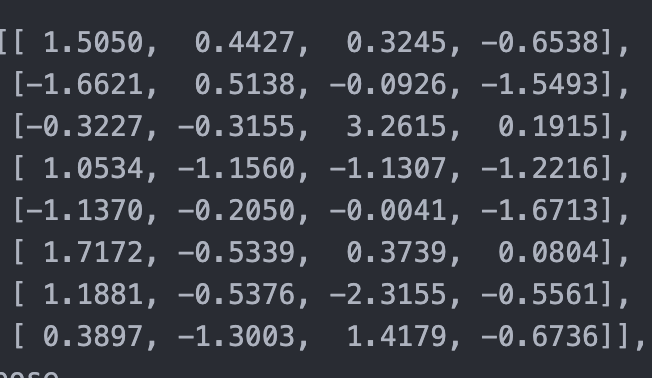
Shape → (8, 4)

Each row represents a token projected into a 4-dimensional query space.

Since the sequence length is 8, we have 8 token representations.

Key Matrix (K)

Before multiplication, we transpose K.

Shape after transpose → (4, 8)

Each column represents a token projected into the same 4-dimensional key space.

Computing Attention Scores

We compute the dot product between Q and $K^{T}$:

(8,4)×(4,8)→(8,8)

This produces the attention score matrix:

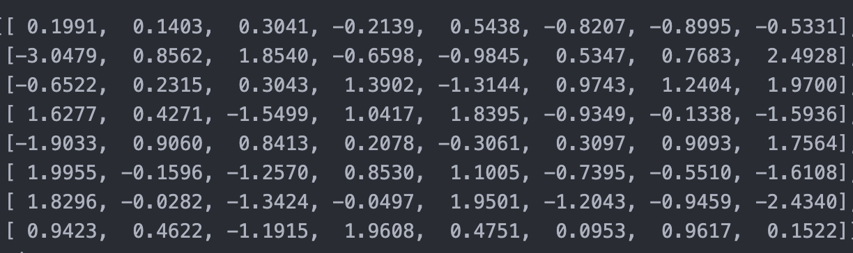
Each element (i, j) measures how strongly token i attends to token j.

Rows are the token asking for information and Columns are the token being attended to. So each row represents how one token distributes its attention across all 8 tokens.

Padding Mask

Unlike the decoder, the encoder does not use causal masking because encoder tokens are allowed to attend to future tokens.

However, we still apply a padding mask.

In our encoder input:

[2, 0, 9, 19, 0, 4, 3, 1]

1 represents the [PAD] token.

Padding tokens are added so that all sequences in a batch have the same length (8 in this case). However, padded positions do not contain meaningful information, so other tokens should not attend to them.

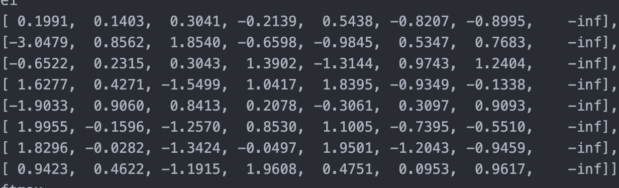
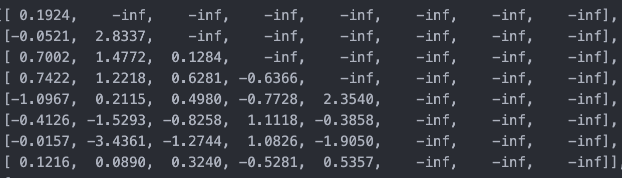
To prevent this, we apply a padding mask that sets attention scores corresponding to [PAD] tokens to a very negative value (-inf).

This ensures that after softmax, padded positions receive probability close to zero.

After applying the mask:

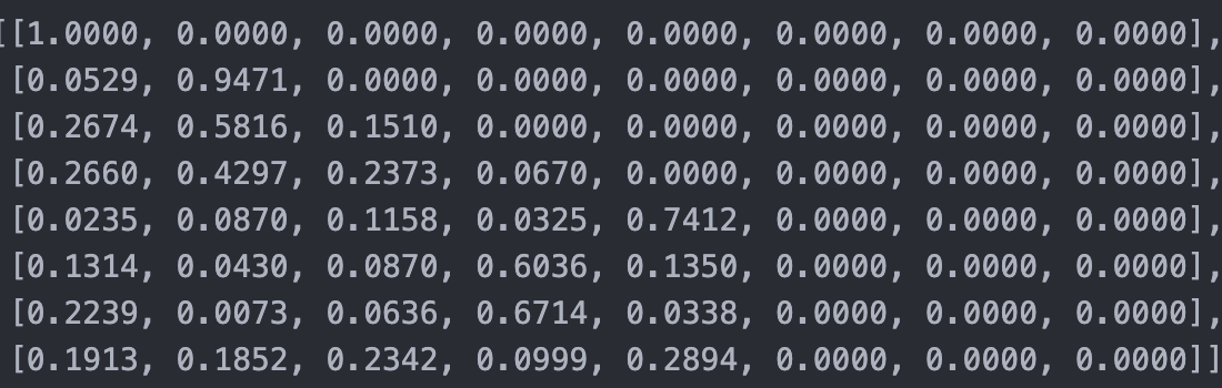
Softmax

Next, we apply softmax to the last dimension

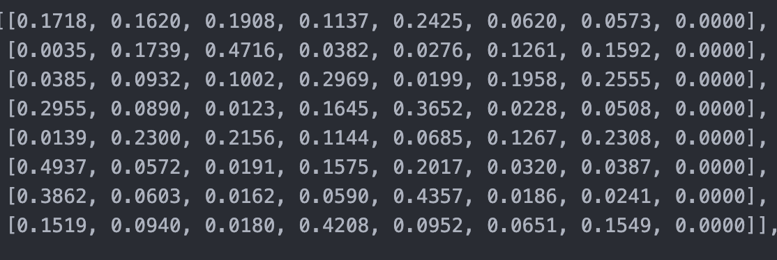
Softmax converts raw attention scores into probabilities.

Now each row sums to 1 and represents how much attention a token gives to every other token.

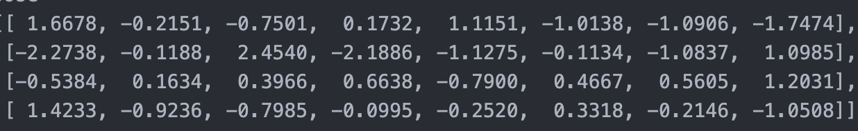
Value Matrix (V)

The value matrix also has original shape (2, 3, 8, 4).

Again, focusing on the first example and first head gives:

Shape → (8, 4)

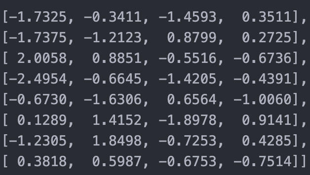
Each row contains the value representation of a token.

Weighted Aggregation

Finally, we multiply the attention probabilities with the value matrix:

(8,8)×(8,4)→(8,4)

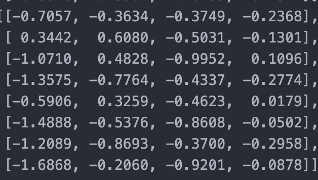
This operation computes a weighted combination of value vectors.

For each token:

• the attention weights determine which tokens are important
• the value vectors provide the information being gathered

The resulting matrix contains updated token representations where each token now carries contextual information from other relevant tokens in the sequence.

# out shape=> (B, H, T, HD) => (B, T, H, HD)
out = out.transpose(1,2).contiguous().view(B, -1, self.emb_dim)
# (C,C) @ (B, T, C)
return out @ self.projection

After attention, we combine all the heads back together and apply a final linear projection so information from all heads can interact with each other.

The attention layer is mainly responsible for communication between tokens. Once tokens exchange information, the Feed Forward Network processes each token independently.

We can think of it like this:

• Attention : tokens communicate with each other
• Feed Forward : each token processes the gathered information independently

The Feed Forward layer expands the embedding dimension, applies a non-linearity, and then projects it back to the original embedding size.

class FeedForward(nn.Module):
    def __init__(self, emb_dim):
        super().__init__()

        self.l1 = nn.Parameter(torch.randn(emb_dim, 4 * emb_dim))
        self.l2 = nn.Parameter(torch.randn(4 * emb_dim, emb_dim))
        self.relu = nn.ReLU()

    def forward(self, x):
        x = x @ self.l1
        x = self.relu(x)
        return x @ self.l2

ResNet helps gradients flow evenly through both the skip connection and the residual branch, which stabilizes training and makes gradient flow healthier. Layer normalization, on the other hand, normalizes activations to have zero mean and unit variance during initialization. As training progresses, it introduces learnable scale and shift parameters that allow the model to adapt the normalized representations while still maintaining stable optimization.

class Resnet(nn.Module):

    def __init__(self, emb_dim):
        super().__init__()
        self.norm = LayerNorm(emb_dim)

    def forward(self, x, sublayer):
        return ( x + sublayer(self.norm(x)))
class LayerNorm(nn.Module):
    def __init__(self, emb_dim):
        super().__init__()
        self.emb_dim = emb_dim
        self.ones = nn.Parameter(torch.ones(1, emb_dim))
        self.zeros = nn.Parameter(torch.zeros(1, emb_dim))

    def forward(self, x):
        xmean = x.mean(dim=-1, keepdim=True)
        xstd = x.std(dim=-1, keepdim=True)
        x = (x-xmean) / (xstd+1e-7)
        x = self.ones * x + self.zeros
        return x

Decoder

From the diagram above we can see Decoder contains 4 components:

• Masked Multi Head Self Attention
• Multi Head Cross Attention
• Resnet and LayerNorm
• FeedForward

The target sequence is shifted to the right so that the model learns to predict the next token using only the previous tokens. A special start token (SOS) is added at the beginning of the target sequence before it is fed into the decoder. This ensures that, during training, the decoder receives past information only, while masked self-attention prevents it from accessing future tokens. As a result, the decoder learns autoregressive generation, producing the output one token at a time.

Masked Multi Head Self Attention

In the decoder, tokens are not allowed to attend to future tokens (t+1). So we apply a causal mask to prevent tokens to attend to future tokens

Example of Causal Masking in Masked Multi Head Self Attention

Attention of shape (8,8)

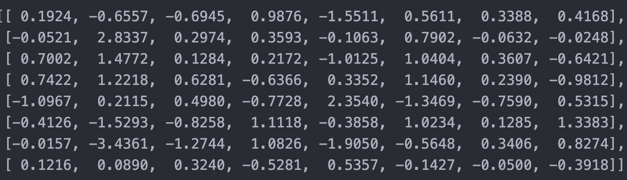
But we dont want token to interact with future tokens and padded tokens

Remeber our decoder input is

[ 2, 0, 668,  92, 4, 1,  1, 1]

and softmax

the rest of the computation is similar to encoder

Cross Multi Head Attention

After masked self-attention, the decoder performs cross attention.

In cross attention:

• Queries come from the Decoder’s self multi head attention
• Keys come from the encoder output
• Values also come from the encoder output

This allows the decoder to look at the source sentence while generating the target sentence.

For English to Nepali translation:

• Encoder processes the English sentence
• Decoder generates the Nepali sentence while attending to the encoder output

Finally, the decoder output is passed through a Feed-Forward Network (FFN), followed by a linear projection layer that maps the representations into the vocabulary space. A softmax layer then produces the probability distribution for predicting the next token.

The Transformer architecture is built by stacking multiple Encoder and Decoder blocks together. Typically, this process is repeated N times, allowing the model to learn increasingly complex representations and relationships within the sequence.

Full Code

class InputEmbeddings(nn.Module):

    def __init__(self, emb_dim, vocab_dim):
        super().__init__()
        self.emb_dim = emb_dim
        self.vocab_dim = vocab_dim
        self.embeddings = nn.Parameter(torch.randn(vocab_dim, emb_dim))

    def forward(self, x):
        return self.embeddings[x] * (self.emb_dim) ** (-1/2)

class PositionalEmbeddings(nn.Module):

    def __init__(self, emb_dim, block_size):
        super().__init__()
        self.block_size = block_size
        self.emb_dim = emb_dim
        self.pe = nn.Parameter(torch.randn(block_size, emb_dim))

    def forward(self, x):

        pe = self.pe[0:x.shape[1], :]
        return x+pe
class LayerNorm(nn.Module):
    def __init__(self, emb_dim):
        super().__init__()
        self.emb_dim = emb_dim
        self.ones = nn.Parameter(torch.ones(1, emb_dim))
        self.zeros = nn.Parameter(torch.zeros(1, emb_dim))

    def forward(self, x):
        xmean = x.mean(dim=-1, keepdim=True)
        xstd = x.std(dim=-1, keepdim=True)
        x = (x-xmean) / (xstd+1e-7)
        x = self.ones * x + self.zeros
        return x

class FeedForward(nn.Module):
    def __init__(self, emb_dim):
        super().__init__()

        self.l1 = nn.Parameter(torch.randn(emb_dim, 4 * emb_dim))
        self.l2 = nn.Parameter(torch.randn(4 * emb_dim, emb_dim))
        self.relu = nn.ReLU()

    def forward(self, x):
        x = x @ self.l1
        x = self.relu(x)
        return x @ self.l2

class Attention(nn.Module):

    def __init__(self, emb_dim, n_head, head_dim):
        super().__init__()
        self.emb_dim = emb_dim
        self.n_head = n_head
        self.head_dim = head_dim
        self.q = nn.Parameter(torch.randn(emb_dim, emb_dim)* (emb_dim)**(-1/2))
        self.k = nn.Parameter(torch.randn(emb_dim, emb_dim) * (emb_dim)**(-1/2))
        self.v = nn.Parameter(torch.randn(emb_dim, emb_dim) * (emb_dim)**(-1/2))
        self.projection = nn.Parameter(torch.randn(emb_dim, emb_dim) * (emb_dim)**(-1/2))

    @staticmethod
    def attention(q, k, v, mask):
        # q=>(B, H, T, HD)
        # k=>(B, H, T, HD)
        # v=>(B, H, T, HD)

        head_dim = q.shape[-1]
        wei = q @ k.transpose(-2, -1) * (head_dim) ** (-1/2)

        # wei=> (B, H, T, HD) @ (B, H, HD, T) => (B, H, T, T)

        if mask is not None:
            wei.masked_fill_(mask==0,float("-inf"))
        wei = wei.softmax(dim=-1)
        # (B, H, T, T)
        # (B, H, T, T)  @ (B, H, T, HD) => (B, H, T, HD)
        return wei@v, wei


    def forward(self, q,k,v, mask):

        B,T,C = q.shape
        q = q @ self.q
        k = k @ self.k
        v = v @ self.v
        q = q.view(q.shape[0], q.shape[1], self.n_head,  self.head_dim).transpose(1,2)
        k = k.view(k.shape[0], k.shape[1], self.n_head,  self.head_dim).transpose(1,2)
        v = v.view(v.shape[0], v.shape[1], self.n_head,  self.head_dim).transpose(1,2)
        out, attn = Attention.attention(q, k, v, mask)

        # out shape=> (B, H, T, HD) => (B, T, H, HD)
        out = out.transpose(1,2).contiguous().view(B, -1, self.emb_dim)
        # (B, T, C) @ (C,C)
        return out @ self.projection

class Resnet(nn.Module):

    def __init__(self, emb_dim):
        super().__init__()
        self.norm = LayerNorm(emb_dim)

    def forward(self, x, sublayer):
        return ( x + sublayer(self.norm(x)))

class EncoderBlock(nn.Module):

    def __init__(self, emb_dim, self_attn, ffd):
        super().__init__()
        self.emb_dim = emb_dim
        self.self_attn = self_attn
        self.ffd = ffd
        self.resnets = nn.ModuleList([Resnet(emb_dim) for _ in range(2)])

    def forward(self, x, src_mask):
        x = self.resnets[0](x, lambda x: self.self_attn(x,x,x, src_mask))
        x = self.resnets[1](x, self.ffd)
        return x

class Encoder(nn.Module):

    def __init__(self,emb_dim, layers):
        super().__init__()
        self.layers = layers
        self.norm = LayerNorm(emb_dim)

    def forward(self, x, mask):
        for layer in self.layers:
            x = layer(x, mask)
        return self.norm(x)

class DecoderBlock(nn.Module):
    def __init__(self,emb_dim, self_attn, cross_attn, ffd):
        super().__init__()
        self.emb_dim = emb_dim
        self.self_attn = self_attn
        self.cross_attn = cross_attn
        self.ffd = ffd
        self.resnet = nn.ModuleList([Resnet(emb_dim) for _ in range(3)])

    def forward(self, x, encoder_output, src_mask, tgt_mask):
        x = self.resnet[0](x, lambda x: self.self_attn(x, x, x, tgt_mask))
        x = self.resnet[1](x, lambda x: self.cross_attn(x, encoder_output, encoder_output, src_mask))
        x = self.resnet[2](x, self.ffd)
        return x

class Decoder(nn.Module):

    def __init__(self, emb_dim, layers):
        super().__init__()
        self.norm = LayerNorm(emb_dim)
        self.layers = layers

    def forward(self, x, encoder_output, src_mask, tgt_mask):
        for layer in self.layers:
            x = layer(x,encoder_output, src_mask, tgt_mask)
        return self.norm(x)

class Projection(nn.Module):
    def __init__(self, emb_dim, vocab_size):
        super().__init__()
        self.proj = nn.Parameter(torch.randn(emb_dim, vocab_size))


    def forward(self, x):
        return x @ self.proj

class Transformer(nn.Module):
    def __init__(self, encoder, decoder, src_embd, tgt_embd, src_pos, tgt_pos, projection_layer):
        super().__init__()
        self.encoder = encoder
        self.decoder = decoder
        self.src_embd = src_embd
        self.tgt_embd = tgt_embd
        self.src_pos = src_pos
        self.tgt_pos = tgt_pos
        self.projection_layer = projection_layer

    def encode_method(self, src, src_mask):
        src = self.src_embd(src)
        src = self.src_pos(src)
        return self.encoder(src, src_mask)


    def decode_method(self, encoder_output, src_mask, tgt, tgt_mask):
        tgt = self.tgt_embd(tgt)
        tgt = self.tgt_pos(tgt)
        # forward(self, x, encoder_output, src_mask, tgt_mask):
        return self.decoder(tgt, encoder_output, src_mask, tgt_mask)

    def projection_method(self, x):
        return self.projection_layer(x)


def build_transformer(src_vocab_size, tgt_vocab_size, src_seq_len, tgt_seq_len, emb_dim, n_layers, n_heads, head_dim):
    src_embedding = InputEmbeddings(emb_dim=emb_dim, vocab_dim=src_vocab_size)
    tgt_embedding = InputEmbeddings(emb_dim=emb_dim, vocab_dim=tgt_vocab_size)

    src_pos = PositionalEmbeddings(emb_dim=emb_dim, block_size=src_seq_len)
    tgt_pos = PositionalEmbeddings(emb_dim=emb_dim, block_size=tgt_seq_len)

    encoder_blocks = []
    for _ in range(n_layers):
        encoder_self_attention_block = Attention(emb_dim=emb_dim, n_head=n_heads, head_dim=head_dim)
        ffd = FeedForward(emb_dim=emb_dim)
        encoder_block = EncoderBlock(emb_dim=emb_dim, self_attn=encoder_self_attention_block, ffd=ffd)
        encoder_blocks.append(encoder_block)

    decoder_blocks = []
    for _ in range(n_layers):
        decoder_self_attn = Attention(emb_dim=emb_dim, n_head=n_heads, head_dim=head_dim)
        decoder_cross_attn = Attention(emb_dim=emb_dim,n_head=n_heads, head_dim=head_dim )
        ffd = FeedForward(emb_dim=emb_dim)
        decoder_block = DecoderBlock(emb_dim=emb_dim, self_attn=decoder_self_attn, cross_attn=decoder_cross_attn, ffd=ffd)
        decoder_blocks.append(decoder_block)

    encoder = Encoder(emb_dim, nn.ModuleList(encoder_blocks))
    decoder = Decoder(emb_dim, nn.ModuleList(decoder_blocks))

    proj = Projection(emb_dim=emb_dim, vocab_size=tgt_vocab_size)

    transformer = Transformer(encoder=encoder, decoder=decoder, src_embd=src_embedding, tgt_embd=tgt_embedding, src_pos=src_pos, tgt_pos=tgt_pos, projection_layer=proj)

    return transformer

transformer = build_transformer(1024, 1024, 8, 8, 12, 1, 3, 4)

PS: The implementation focuses on clarity and understanding of the Transformer’s internal operations rather than performance optimizations or computational efficiency.