RNN, LSTM and the need for Attention
In Markov Sequence Model, we encounterd several major challenges:
- The transition tables grow exponentially as the sequence length increases.
- The models tend to overfit the training data as well as cause sparsity in the table
In this blog post, I will discuss Recurrent Neural Network (RNN), Long Short-Term Memory Network (LSTM), and the need for Attention
Encoding
There are several ways to represent text numerically:
- Character-level encoding — each character is mapped to a unique number.
a => 0, b => 1 ... and so on
- Word embeddings — each word is mapped to a vector representation.
hello => 0, world => 1 ... and so on
- Sentence embeddings — entire sentences are converted into vectors.
Hello My name is Shusanket => 1, I am from Nepal => 2
- And many more approaches.
In this blog post, I will focus on Byte Pair Encoding (BPE), which sits between character-level and word-level encoding.
Byte Pair Encoding (BPE)
Byte Pair Encoding is a tokenization algorithm that transforms raw text into subword tokens.
Suppose we have the following string:
"abaabbc"
If we encode this string using UTF-8, we get the following byte sequence:
[97, 98, 97, 97, 98, 98, 99]
BPE operates at the byte level. The process begins by encoding the text using formats such as UTF-8, UTF-16, or UTF-32. After encoding, the algorithm repeatedly finds the most frequent pair of adjacent bytes and merges them into a new token.
In the example above, the pair:
[97, 98]
appears twice, while the other pairs appear only once. Since byte values occupy the range 0–255, the newly merged token is assigned the next available token ID, such as 256.
After the merge, the sequence becomes:
[256, 97, 256, 98, 99]
The algorithm then repeats this process for a predefined number of merges, gradually building larger and more meaningful subword tokens.
This approach is powerful because it balances the advantages of both character-level and word-level tokenization:
- Character-level models can handle unseen words but produce very long sequences.
- Word-level models are efficient but struggle with unknown or rare words.
- BPE provides a middle ground by learning commonly occurring subword units.
Code
def get_stats(ids, counts =None):

    counts = {} if counts is None else counts
    for pair in zip(ids, ids[1:]):
        counts[pair] = counts.get(pair, 0)+1
    return counts

def merge(tokens, pair, new_id):
    i = 0
    new_tokens = []
    while i<len(tokens):
        if tokens[i]==pair[0] and i+1<len(tokens) and tokens[i+1]==pair[1]:
        new_tokens.append(new_id)
        i+=2
        else:
        new_tokens.append(tokens[i])
        i+=1
    return new_tokens

def train(text, vocab_size):
    num_merges = vocab_size-256
    text_chunks = re.findall(GPT4_SPLIT_PATTERN, text)
    ids = [list(ch.encode("utf-8")) for ch in text_chunks]

    merges = {}
    vocab = {idx:bytes([idx]) for idx in range(256)}
    for i in range(num_merges):
        stats = {}
        for k , chunk_ids in enumerate(ids):
            get_stats(chunk_ids, stats)
        pair = max(stats, key=stats.get)
        idx = 256+i
        ids = [merge(chunk_ids, pair, idx) for chunk_ids in ids]
        merges[pair] = idx
        print(f"merging {pair} to {idx}")
        print(f"{i}/{num_merges}")
        vocab[idx] = vocab[pair[0]]+vocab[pair[1]]
    return merges, vocab

def decode(ids):
    ids = [i.item() for i in ids]
    bytes_stream = b"".join(vocab[idx] for idx in ids)
    text = bytes_stream.decode("utf-8", errors='replace')
    return text

def encode(text):
    ids = list(text.encode("utf-8"))
    while len(ids)>=2:
        stats = get_stats(ids)
        pair = min(stats, key=lambda p:merges.get(p, float("inf")))
        if pair not in merges:
            break
        idx = merges.get(pair)
        ids = merge(ids, pair,idx)
    return ids
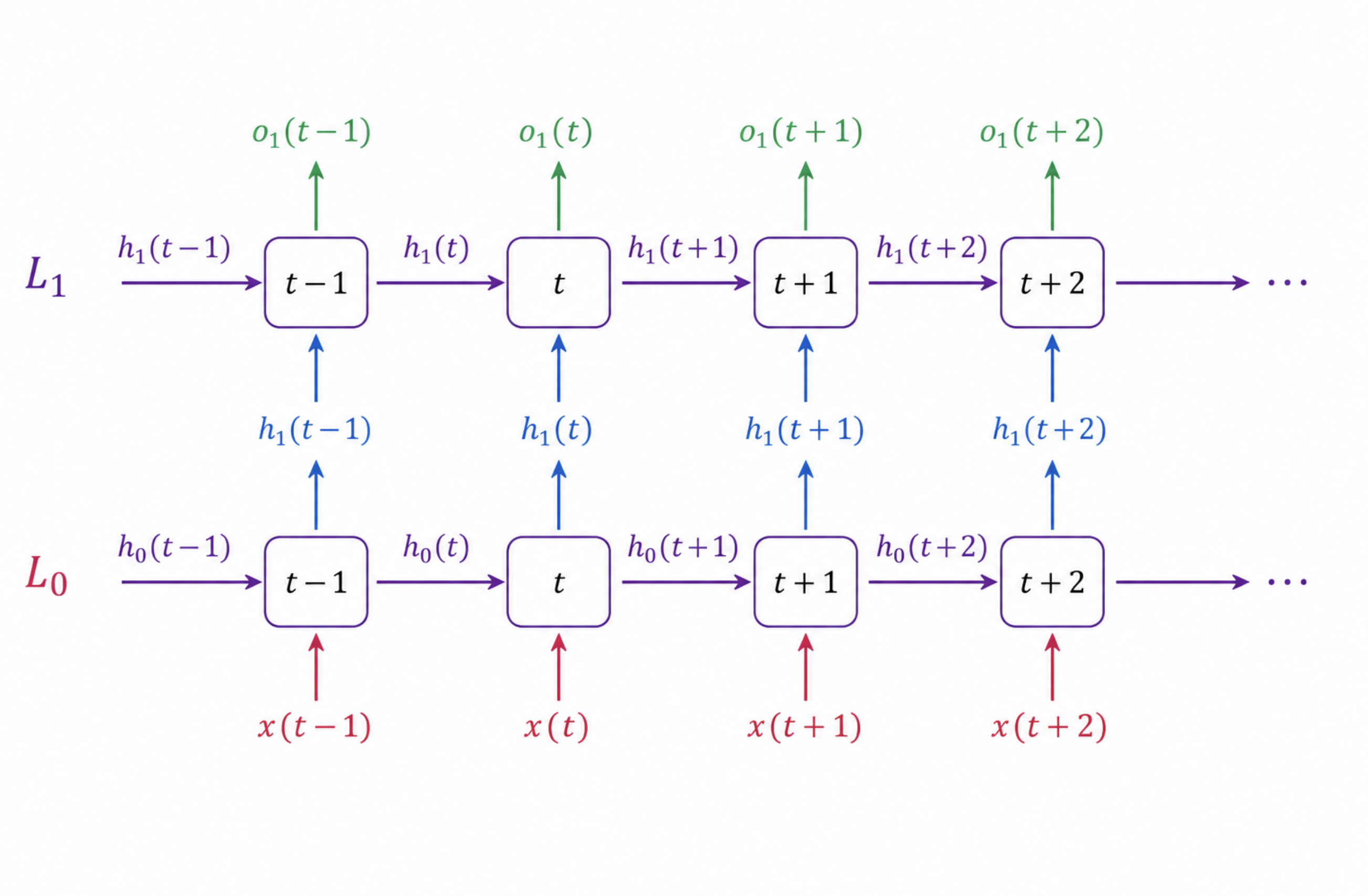
RNN model
Recurrent Neural Networks (RNNs) are a type of neural network designed for processing sequential data such as text, speech, and time-series data.
Unlike traditional neural networks, RNNs have a memory mechanism that allows information from previous inputs to influence future outputs. This makes them especially useful for tasks where context and order matter.
An RNN processes data one element at a time while maintaining a hidden state that carries information from previous steps.
At each time step:
- The current input is processed.
- The previous hidden state is combined with the current input.
- A new hidden state is generated.
- The output is produced.
Mathematical Representation
\[h_t = f(W x_t + U h_{t-1} + b)\]Where:
- $(x_t)$ = current input
- $(h_{t-1})$ = previous hidden state
- $(h_t)$ = current hidden state
- $(W, U)$ = weight matrices
- $(b)$ = bias
- $(f)$ = activation function such as tanh or ReLU
The hidden state acts as the memory of the network.
RNN Code
class LayerNormalization(nn.Module):
    def __init__(self, embdim):
        super().__init__()
        self.mul = nn.Parameter(torch.ones(1, embdim))
        self.add = nn.Parameter(torch.zeros(1, embdim))

    def forward(self, x):
        xmean = x.mean(axis=-1, keepdim=True)
        xstd = x.std(axis=-1, keepdim=True)
        x = (x-xmean) / ((xstd+1e-07) ** 1/2)
        x = self.mul * x + self.add
        return x
# multi layer RNN

class RNN(nn.Module):
    def __init__(self, emb_dim, vocab_size, hidden_dim, block_size, n_layers):
        super().__init__()
        self.emb_dim = emb_dim
        self.vocab_size = vocab_size
        self.n_layers = n_layers
        self.embedding = nn.Parameter(torch.randn(vocab_size, emb_dim)* (self.vocab_size) ** (-1/2))
        self.hidden_dim = hidden_dim
        self.block_size = block_size
        self.vocab_size = vocab_size

        self.input_to_hidden = nn.ParameterList(
                [nn.Parameter(torch.randn(self.emb_dim, self.hidden_dim) * (self.emb_dim)**(-1/2))] +
                [nn.Parameter(torch.randn(self.hidden_dim, self.hidden_dim) * (self.hidden_dim) ** (-1/2) ) for _ in range(self.n_layers - 1)]
            )
        self.hidden_to_hidden = nn.Parameter(torch.randn(self.n_layers, self.hidden_dim, self.hidden_dim)* (self.hidden_dim)**(-1/2))
        self.hidden_to_output = nn.Parameter(torch.randn(self.hidden_dim, self.vocab_size) * (self.hidden_dim)**(-1/2))

        self.LayerNorms = nn.ModuleList(
            [LayerNormalization(self.hidden_dim) for _ in range(self.n_layers)]
        )
        self.dropout = nn.Dropout(0.2)


    def forward(self, x, batch_size, traintest, hidden_layer = None ):

        x = self.embedding[x]
        if hidden_layer is None:
            hidden_prev = torch.zeros((self.n_layers, batch_size, self.hidden_dim))


        out = []
        x = x.transpose(0, 1)
        hidden_mem = []

        for t in range(x.shape[0]):

            hidden_curr = []

            for l in range(self.n_layers):

                if l==0:
                    curr_x = x[t]
                else:
                    curr_x = hidden_curr[l-1]

                x_ih = curr_x @ self.input_to_hidden[l]

                x_hh = hidden_prev[l] @ self.hidden_to_hidden[l]
                x_nn = x_hh+x_ih
                x_new = (torch.tanh(self.LayerNorms[l](x_nn)))

                if traintest=="train":
                    if l==self.n_layers-1:
                        x_nn.retain_grad()
                        hidden_mem.append(x_nn)

                hidden_curr.append(x_new)

            hidden_curr = torch.stack(hidden_curr)

            hidden_prev = hidden_curr
            out.append(hidden_prev[-1])


        out = torch.stack(out)
        out = out @ self.hidden_to_output
        out = out.transpose(0,1).contiguous()
        return hidden_mem, out

import matplotlib.pyplot as plt
for k in range(1):
    lossi = []
    for _ in range(dataiter):
        if _%100==0:
            print(f"{k}/10->{_}/{dataiter} ")
        x,y = generate_batch(ids_train, block_size=block_size, batch_size=batch_size)
        hidden, logits = model(x, batch_size=batch_size, traintest = "train")
        # print(logits.shape)
        logits = logits.view(-1, logits.shape[-1])
        y = y.view(-1)

        # OR just look at the final logit to make exploding/vanishing gradient visible

        # logits_last = logits[:, -1, :]   # shape: [batch, vocab]
        # y_last = y[:, -1]
        # logits_last = logits_last.view(-1, logits_last.shape[-1])

        loss = F.cross_entropy(logits, y)
        optimizer.zero_grad()
        loss.backward()
        optimizer.step()
        lossi.append(loss.item())

        if _ == 0:
            gradloss = []
            for _ in range(len(hidden)):
                    gradloss.append(hidden[_].grad.norm().item())
            print("plotting gradloss")
            plt.plot(gradloss)
            plt.show()

    lossi = torch.tensor(lossi)
    losstrainig.append(lossi.mean().item())

    print(f" training loss => {lossi.mean()}")

    with torch.no_grad():
            losste = []
            model.eval()
            for _ in range(testiter):
                x,y = generate_batch(ids_test, block_size=block_size, batch_size=batch_size)
                _, logits = model(x, batch_size, traintest ="test")
                logits = logits.view(-1, logits.shape[-1])
                print(logits.mean())
                y = y.view(-1)
                loss = F.cross_entropy(logits, y)
                losste.append(loss.item())
            losste = torch.tensor(losste)
            print(f"test loss {losste.mean().item()}")
            losstest.append(losste.mean().item())
            model.train()
Since I am applying Layer Norm, I have omitted bias parameter
Exploding and Vanishing Gradient
In the above implementation, I computed the loss at every timestep. This provides strong local gradient signals because each hidden state directly contributes to a nearby loss term. As a result, the gradients do not need to propagate across long temporal distances, which masks the vanishing gradient phenomenon. To properly observe vanishing gradients, the loss should be computed only from the final timestep logits. In that case, the gradient must propagate backward through the entire sequence of recurrent transitions, making the exponential decay of gradients across time visible.
Exploding and vanishing gradients are among the major bottlenecks in Recurrent Neural Network (RNN) architectures. These problems occur during the backpropagation process when gradients are propagated through many time steps. In the case of vanishing gradients, the gradient values become extremely small, making it difficult for the network to learn long-term dependencies in sequential data. As a result, the model fails to retain important information from earlier inputs. On the other hand, exploding gradients occur when gradient values grow excessively large, causing unstable learning and significant fluctuations in weight updates.
Exploding Gradient
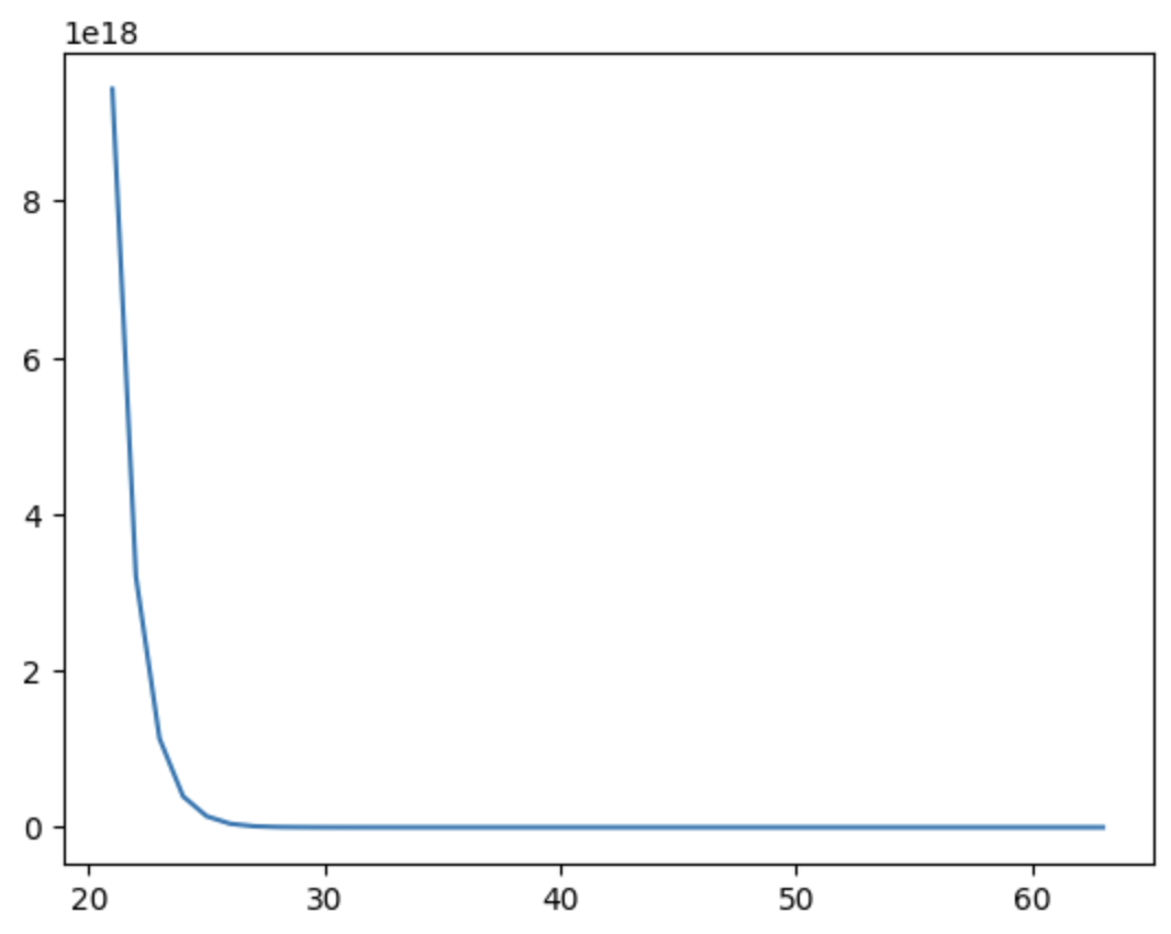
The graph above illustrates the exploding gradient problem, where the x-axis represents the time-step layers and the y-axis represents the gradient norm at each time step. During backpropagation through time, the gradient values increase exponentially as they propagate across layers. As a result, the gradients become extremely large and may skyrocket toward infinity, causing unstable learning and drastic weight updates. This instability can prevent the RNN from converging properly and may lead to poor model performance during training.
Vanishing Gradient
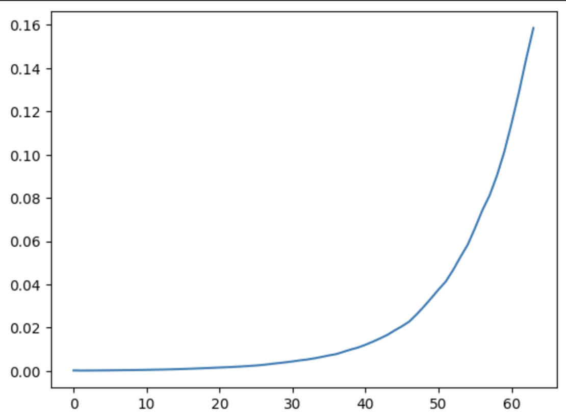
It is very difficult for the network to preserve information over long time steps as the hidden state is repeatedly updated and overwritten at every time step, causing important earlier information to gradually disappear.
This is where novel architecture Long Short-Term Memory (LSTM) network and Attention architecture comes into play.
LSTMs use multiple memory cells and gating mechanisms to selectively retain or forget information over time. Similarly, attention mechanisms help gradients flow more effectively by creating direct connections between relevant input and/or output states, allowing the model to focus on important information without relying solely on long sequential propagation through hidden states.
LSTM
LSTM is a part of RNN archtiecture with some additional gates which helps to regulate the flow of information through a carefully designed memory mechanism.
Instead of blindly propagating information through time, an LSTM selectively decides:
- what information should be remembered,
- what information should be forgotten,
- what new information should be stored,
- and what information should be exposed as output.
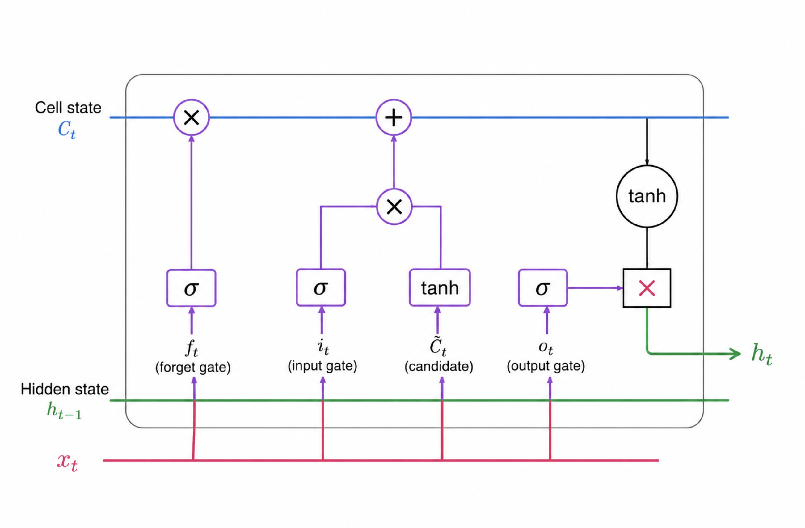
The Two Core States of an LSTM
At every time step, an LSTM maintains two different internal representations:
Cell State ($C_t$)
The cell state acts as the long-term memory of the network. It carries important information across multiple time steps and flows almost linearly through the architecture. This linear pathway allows information to persist over long sequences.
Hidden State ($h_t$)
The hidden state represents the short-term working memory of the network. It contains information relevant to the current time step and is also passed to the next LSTM cell.
While the hidden state changes rapidly over time, the cell state evolves more carefully and selectively.
Information Flow Through the LSTM
At each time step $t$, the LSTM receives:
\[x_t, \quad h_{t-1}, \quad C_{t-1}\]where:
- $x_t$ is the current input,
- $h_{t-1}$ is the previous hidden state,
- $C_{t-1}$ is the previous cell state.
Using these inputs, the LSTM computes the updated hidden state $h_t$ and updated cell state $C_t$.
The flow of information is controlled by three gates:
- Forget Gate
- Input Gate
- Output Gate
Each gate uses sigmoid activations that generate values between 0 and 1, effectively acting as control valves for information flow.
Forget Gate
The forget gate determines which information from the previous cell state should be retained and which should be discarded.
The forget gate is computed as:
\[f_t = \sigma(W_{fh} h_{t-1} + W_{fx} x_t + bias(es))\]The sigmoid activation produces values between 0 and 1:
- values close to 0 indicate information that should be forgotten,
- values close to 1 indicate information that should be preserved.
The forget gate filters the previous cell state through element-wise multiplication:
\[f_t \odot C_{t-1}\]This allows the network to selectively remove irrelevant information from memory.
Input Gate
After removing unnecessary information, the LSTM determines what new information should be stored in memory.
The input gate consists of two components.
First, the gate determines which information should be updated:
\[i_t = \sigma(W_{ih} h_{t-1} + W_{ix} x_t + bias(es))\]Next, the network generates memory values to be updated:
\[% \tilde{C}_t = \tanh(W_c[h_{t-1}, x_t] + b_c) \tilde{C}_t = \tanh(W_{ch} h_{t-1} + W_{cx} x_t + bias(es))\]The candidate state contains new information that may be added to memory.
Updating the Cell State
The updated cell state combines retained old memory with selected new information:
\[C_t = f_t \odot C_{t-1} + i_t \odot \tilde{C}_t\]This equation represents the core memory update mechanism of the LSTM.
The first term preserves useful information from the past, while the second term introduces newly learned information.
Because the cell state evolves through a relatively stable pathway, gradients can propagate more effectively during training. This enables the network to learn long-range dependencies that traditional RNNs struggle to capture.
Output Gate
The final stage determines what information should be exposed as the hidden state.
First, the output gate computes a mask:
\[% o_t = \sigma(W_o[h_{t-1}, x_t] + b_o) o_t = \sigma(W_{oh} h_{t-1} + W_{ox} x_t + bias(es))\]Then the hidden state is generated as:
\[h_t = o_t \odot \tanh(C_t)\]The hidden state serves two purposes:
- it becomes the output of the current time step,
- and it is passed to the next LSTM cell.
While the cell state stores long-term memory internally, the hidden state acts as the externally visible representation of that memory.
Why LSTMs Are Effective
Traditional RNNs repeatedly overwrite their internal representations, making it difficult to preserve information over long sequences.
LSTMs solve this problem through gated memory control.
By learning what to forget, what to store, and what to expose, LSTMs can effectively model long-term dependencies in sequential data.
Gradient of the Cell State over Time
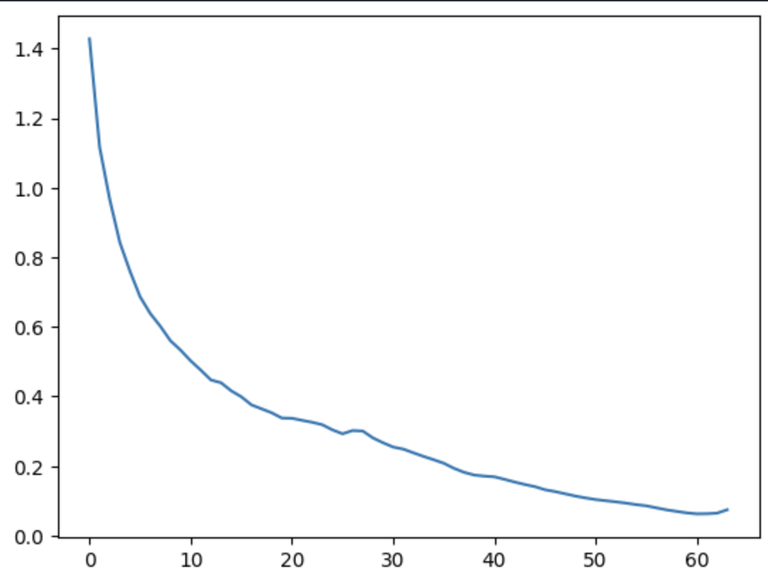
In LSTM, the gradients can still suffer from vanishing and/or exploding gradient problems, but the issue is much less severe compared to traditional RNNs because of the cell state and gating mechanisms. For exploding gradients, techniques such as gradient clipping, proper weight initialization, and normalization methods are commonly used. However, vanishing gradients are more difficult to handle because, over long sequences, the model struggles to retain information from earlier time steps.
This is where the attention mechanism plays a major role. Instead of forcing the network to compress all past information into a single/multiple hidden state, attention allows the model to directly focus on the most relevant parts of the input sequence when making predictions. In other words, the model no longer depends entirely on long-term gradient flow to remember earlier information.
LSTM Code
class LSTM(nn.Module):

    def __init__(self, emb_dim, vocab_size, hidden_dim, n_layers):
        super().__init__()
        self.emb_dim = emb_dim
        self.vocab_size = vocab_size
        self.hidden_dim = hidden_dim
        self.n_layers = n_layers

        self.embeddings = nn.Parameter(torch.randn(self.vocab_size, self.emb_dim) * (self.vocab_size) ** (-1/2))


        self.i_i =  nn.ParameterList(
                [nn.Parameter(torch.randn(self.emb_dim, self.hidden_dim) * (self.emb_dim)**(-1/2))] +
                [nn.Parameter(torch.randn(self.hidden_dim, self.hidden_dim) * (self.hidden_dim) ** (-1/2) ) for _ in range(self.n_layers - 1)]
            )
        self.h_i = nn.Parameter(torch.randn(self.n_layers, self.hidden_dim, self.hidden_dim) * (self.hidden_dim) ** (-1/2))


        self.i_ff = nn.ParameterList(
                [nn.Parameter(torch.randn(self.emb_dim, self.hidden_dim) * (self.emb_dim)**(-1/2))] +
                [nn.Parameter(torch.randn(self.hidden_dim, self.hidden_dim) * (self.hidden_dim) ** (-1/2) ) for _ in range(self.n_layers - 1)]
            )

        self.h_ff = nn.Parameter(torch.randn(self.n_layers, self.hidden_dim, self.hidden_dim) * (self.hidden_dim) ** (-1/2) )


        self.i_g =  nn.ParameterList(
                [nn.Parameter(torch.randn(self.emb_dim, self.hidden_dim) * (self.emb_dim)**(-1/2))] +
                [nn.Parameter(torch.randn(self.hidden_dim, self.hidden_dim) * (self.hidden_dim) ** (-1/2) ) for _ in range(self.n_layers - 1)]
            )

        self.h_g = nn.Parameter(torch.randn(self.n_layers, self.hidden_dim, self.hidden_dim) * (self.hidden_dim) ** (-1/2) )


        self.i_o = nn.ParameterList(
                [nn.Parameter(torch.randn(self.emb_dim, self.hidden_dim) * (self.emb_dim)**(-1/2))] +
                [nn.Parameter(torch.randn(self.hidden_dim, self.hidden_dim) * (self.hidden_dim) ** (-1/2) ) for _ in range(self.n_layers - 1)]
            )
        self.h_o = nn.Parameter(torch.randn(self.n_layers, self.hidden_dim, self.hidden_dim) * (self.hidden_dim) ** (-1/2) )

        self.LayerNorms = nn.ModuleList(
            [
                   nn.ModuleList(
                       LayerNormalization(self.hidden_dim) for _ in range(4) )
                for _ in range(self.n_layers)

            ]

        )


        self.proj = nn.Parameter(torch.randn(self.hidden_dim, self.vocab_size) * (self.hidden_dim) ** (-1/2))

    def forward(self, x,  batch_size, traintest = "train", hidden=None):
        # always batch first

        # x shape (B, T)
        x = self.embeddings[x]
        # x shape (T, B, E)
        x = x.transpose(0,1)

        if hidden is None:
            hidden_prev = torch.zeros(self.n_layers, batch_size, self.hidden_dim)
            cell_prev = torch.zeros(self.n_layers, batch_size, self.hidden_dim)

        out = []
        hidden_mem = []
        for t in range(x.shape[0]):
            h_curr = []
            c_curr = []
            for l in range(self.n_layers):
                if l==0:

                    curr_x = x[t]
                else:
                        curr_x = h_curr[-1]

                # curr shape => (B, E)

                # forget_gate

                # shapes:
                # curr_x => (B,E),
                # self.i_ff => (L, E, H),
                # self.i_ff[L] => (E, H),
                # hidden_prev => (L, B, H)
                # hidden_prev[l]=> (B, H)
                # self.h_ff => (L, H, H)
                # self.h_ff[l] => (H, H)

                # first iter
                # (B,E) @ (E, H) + (B, H) @ (H,H)
                # (B, H) + (B, H) => (B, H)

                #second iter+
                # curr => (B,H)
                # (B,H) @ (E, H) + (B, H) @ (H,H)
                # (B,H) + (B,H) => (B,H)

                f_gate = torch.sigmoid(self.LayerNorms[l][0](curr_x @ self.i_ff[l] + hidden_prev[l] @ self.h_ff[l]))


                # first iter
                # input gate
                # (B, E) @ (E, H) + (B, H) @ (H, H)
                # (B, H) + (B, H) => (B, H)

                # second iter+
                # (B,H) @ (E, H) + (B, H) @ (H, H)

                i_gate = torch.sigmoid(self.LayerNorms[l][1](curr_x @ self.i_i[l] + hidden_prev[l] @ self.h_i[l]))

                # first iter
                # (B,E) @ (E, H) + (B, H) @ (H,H)
                # (B, H) + (B, H) => (B, H)

                # second iter +
                # (B,H) @ (H, H) + (B, H) @ (H,H)
                # (B, H) + (B, H) => (B, H)

                g_gate = torch.tanh(self.LayerNorms[l][2](curr_x @ self.i_g[l] + hidden_prev[l] @ self.h_g[l]))

                #
                # (B, H) * (B, H) + (B, H) * (B, H)
                # (B, H) + (B, H) => (B, H)
                curr_cell = f_gate * cell_prev[l] + i_gate * g_gate
                if traintest =="train":
                    if l==self.n_layers-1:
                        curr_cell.retain_grad()
                        hidden_mem.append(curr_cell)

                # output_gate
                # (B, E) @ (E, H) + (B, H) @ (H,H)
                # (B, H) + (B, H) => (B, H)

                # second iter +
                # (B,H) @ (H,H) + (B, H) @ (H,H)
                # (B,H) + (B,H) => (B,H)
                o_gate = torch.sigmoid(self.LayerNorms[l][3](curr_x @ self.i_o[l] + hidden_prev[l] @ self.h_o[l]))

                # (B, H) * (B, H)
                # (B, H)
                curr_hidden = torch.tanh(curr_cell) * o_gate

                c_curr.append(curr_cell)
                h_curr.append(curr_hidden)

            hidden_prev = torch.stack(h_curr)
            cell_prev = torch.stack(c_curr)
            out.append(hidden_prev[-1])

        out = torch.stack(out)
        output = out @ self.proj
        output = output.transpose(0,1).contiguous()
        return hidden_mem, output